Range, variance and standard deviation as measures of dispersion:
(Khan Academy Video)Variance measures how far a set of numbers is spread out. (A variance of zero indicates that all the values are identical.) A small variance indicates that the data points tend to be very close to the mean (expected value) and hence to each other, while a high variance indicates that the data points are very spread out from the mean and from each other.
The Variance is defined as: The average of the squared differences from the Mean.
The formula for measuring an unbiased estimate of the population variance from a fixed sample of n observations is the following:
(s2) = Σ [(xi - x̅)2]/n - 1
The formula for calculating the variance in an entire population is the same as this one except the numerator is n, not n - 1, but it should not be used any time you are working with a finite sample of observations. Here's what the parts of the formula for calculating variance mean:
- s2 = Variance
- Σ = Summation, which means the sum of every term in the equation after the summation sign.
- xi = Sample observation. This represents every term in the set.
- x̅ = The mean. This represents the average of all the numbers in the set.
- n = The sample size. You can think of this as the number of terms in the set.
The standard deviation shows how much variation or dispersion from the average exists. It represents the average deviation from the mean. A low standard deviation indicates that the data points tend to be very close to the mean (also called expected value); a high standard deviation indicates that the data points are spread out over a large range of values.
With a normal or bell-shaped distribution, 1 SD holds 68% of values, 2 SDs hold 95% of values, and 3 SDs hold 99.7% of values. In a normal distribution, the mean = median = mode (mean is the average value, median is the middle value, and mode is the most common value).
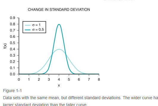
Figure 1-1Data sets with the same mean, but different standard deviations. The wider curve has a larger standard deviation than the taller curve.
● Example: Normal body temperature will have a small SD because an individual’s anterior and posterior hypothalamus maintains temperature homeostasis within a very limited range. Blood sugars, on the other hand, will have a larger SD because glycemic loads change throughout the day.
The standard deviation is represented by the Greek letter sigma, σ.
The standard deviation is the square root of its variance of a random variable, statistical population, data set, or probability distribution. It is algebraically simpler though in practice less robust than the average absolute deviation. A useful property of the standard deviation is that, unlike the variance, it is expressed in the same units as the data. Note, however, that for measurements with percentage as the unit, the standard deviation will have percentage points as the unit.
In addition to expressing the variability of a population, the standard deviation is commonly used to measure confidence in statistical conclusions. For example, the margin of error in polling data is determined by calculating the expected standard deviation in the results if the same poll were to be conducted multiple times. The reported margin of error is typically about twice the standard deviation—the half-width of a 95 percent confidence interval. In science, researchers commonly report the standard deviation of experimental data, and only effects that fall much farther than two standard deviations away from what would have been expected are considered statistically significant—normal random error or variation in the measurements is in this way distinguished from causal variation.
Confidence interval: When you take a set of data and calculate a mean, you want to say that the result is equivalent to the mean of the whole population, but usually the two values are not exactly equal. The confidence interval (usually set at 95%) says that you are 95% confident that the mean of the population is within a certain range (generally within 2 SD of your experimental or derived mean using an adjustment for the sample size). A confidence interval (confidence limits) expressed as 76 < X < 84 = 0.95 means that you are 95% certain that the mean for the whole population (X) is between 76 and 84.
When only a sample of data from a population is available, the term standard deviation of the sample or sample standard deviation can refer to either the above-mentioned quantity as applied to those data or to a modified quantity that is a better estimate of the population standard deviation (the standard deviation of the entire population).
CASE SCENARIO
A child scores 140 on an IQ test. A review of the literature reveals that the mean IQ in the child’s community is 100, with an SD of 20. How does the child’s score compare with that of other children? The child did better on the examination than 97.5% of children in the community. The child scored 2 standard deviations above the mean, which holds 95% of the values. Because 2.5% fall on each end of the bell-shaped curve, the child did better on the examination than 97.5% of children in the community.
The standard error is an estimate of the standard deviation of a statistic. This lesson shows how to compute the standard error, based on sample data.1
The standard error is important because it is used to compute other measures, like confidence intervals and margins of error.
Reference
1. http://stattrek.com/estimation/standard-error.aspx?Tutorial=AP
Normal distribution
Also known as a gaussian distribution or bell-shaped curve. A probability function in which values are symmetrically distributed around a central value, and the mean, median, and mode are equal .
In a normal distribution, 1 SD accounts for 68% of all values, 2 SDs account for 95% of all values, and 3 SDs account for 99.7% of all values—the 68-95-99 rule ( Fig. 1-2 ). The area under the curve is 1 (100%).
In a normal distribution, 1 standard deviation (SD) accounts for 68% of all values, 2 SDs account for 95% of all values, and 3 SDs account for 99% of all values.(From Marshall WJ, Bangert SK. Clinical Chemistry. 6th ed. Philadelphia: Elsevier; 2008.)● Example: The intelligence quotient (IQ) test is constructed to follow a normal distribution with a mean of 100 and SD of 15. That means that 95% of the population (2 SDs) will have an IQ between 70 and 130. Of clinical import, mental retardation is defined as an IQ of < 70.
❍ Bimodal distribution:
A distribution with two modes.
● Example: The incidence of Crohn’s disease displays a bimodal distribution with the first peak between 15 and 30 years of age and the second peak between 60 and 80 years of age.
❍ Negative skew:
An asymmetrical distribution in which a tail on the left indicates that mean < median < mode . The tail is due to outliers on the left side of the curve.
● Example: A graphic representation of age at death would show a negative skew, with most people clustered at the right end of the distribution and relatively few dying at a younger age ( Fig. 1-3A ).
Figure 1-3A, Negative skew. B, Positive skew.(From Jekel JF, Katz DL, Wild JG, Elmore DMG. Epidemiology, Biostatistics, and Preventive Medicine. 3rd ed. Philadelphia: Elsevier; 2007.)❍ Positive skew:
An asymmetrical distribution, in which a tail on the right side indicates that mean > median > mode . The tail is due to outliers on the right side of the curve.
● Example: A graphic representation of age at initiation of smoking would display positive skew. Most people would be clustered around their late teens, but a small number of middle-aged and older adults, who initiated smoking later in life, create a positive tail ( Fig. 1-3B ).
Skewed distribution: A positive skew is asymmetry with an excess of high values (tail on right, mean > median > mode); a negative skew is asymmetry with an excess of low values (tail on left, mean < median < mode). Because positive and negative skews ( Fig. 1-3 ) are not normal distributions, standard deviation and mean are less meaningful values.
Figure 1-3Group A demonstrates a negative skew (tail on the left), group B has a normal distribution, and group C has a positive skew (tail on the right).
Content 5
The distribution of variation in heart rate to deep breathing and the Valsalva ratio from the study by Gelber and colleagues (1997) is given in Figure 1 in their article and is reproduced below in Figure 13–7. What is the best method to find the normal range of values for the Valsalva ratio?
+Figure 13–7.
Graphic Jump Location+
A: Distribution of normative values for heart rate variation to deep breathing (VAR) and B: Valsalva ratio (VAL) for the entire study population. (Reproduced, with permission, from Figure 1 in Gelber DA, Pfeifer M, Dawson B, Shumer M: Cardiovascular autonomic nervous system tests: Determination of normative values and effect of confounding variables. J Auton Nerv Syst 1997;62:40–44.)
The distribution of variation in heart rate to deep breathing and the Valsalva ratio from the study by Gelber and colleagues (1997) is given in Figure 1 in their article and is reproduced below in Figure 13–7. What is the best way to describe the distribution of these values?
+Figure 13–7.
Graphic Jump Location+A: Distribution of normative values for heart rate variation to deep breathing (VAR) and B: Valsalva ratio (VAL) for the entire study population. (Reproduced, with permission, from Figure 1 in Gelber DA, Pfeifer M, Dawson B, Shumer M: Cardiovascular autonomic nervous system tests: Determination of normative values and effect of confounding variables. J Auton Nerv Syst 1997;62:40–44.)
Click Here for Answer.
Content 3
Digital World Medical School


